
Suppose a model loads and answers a short prompt without trouble. Then a long conversation arrives, or several users start generating at the same time, and the server runs out of memory. The weights are the same. More memory is now needed for the work done during those requests.
Part of that memory holds the KV cache, data kept from earlier tokens so the model can reuse it. Its size follows directly from how attention works and how the model generates text. Unlike the weights in a model file, this data is built while the model runs.
Why the next token depends on earlier ones
A token is a piece of the model's input, often a word, part of a word or punctuation. The models covered here are Transformer decoders with causal attention. They generate text autoregressively. That means each new token is predicted from the tokens already in the context, including the prompt and the output produced so far.
The model first processes the prompt and returns scores for the next possible tokens. The serving engine chooses one, adds it to the context and asks for the next prediction. The same loop continues until generation stops. The Transformer walkthrough follows a complete run through these steps.
Every prediction needs information from the existing context. One way to get it is to process that context again on each pass. A cache gives the engine another option. It keeps part of the earlier attention calculations and reuses them when processing the new position.
This makes the KV cache central to efficient generation in these models. Autoregression still works without it, but the engine repeats calculations for tokens it has already processed. To see which results are worth keeping, we need to look inside attention.
What queries, keys and values do
At each layer, a token is represented by a vector, a list of numbers. Attention lets the current position gather information from other positions. It does this through three learned transformations called query, key and value projections. Each projection multiplies the input vector by a matrix, a table of learned numbers stored in the model.
Attention is split into heads. Each head makes its own comparisons and produces its own output vector. For one head at position , let be the input vector. The three projections give
The matrices , and stay fixed during inference. The resulting vectors depend on the tokens being processed. The lowercase letters above describe one position. Uppercase Q, K and V usually refer to collections of those vectors. Some models also transform queries and keys to include position information, for example with RoPE. The equations above show only the projections.
The query describes what the current position will compare against. Each key provides the numbers used in that comparison. Each value provides information that can be passed into the result. All positions produce keys and values, including the current one.
The head compares the current query with each available key using a dot product. It multiplies the numbers in matching positions in the two vectors, then adds the results. This gives one score per position. A larger score gives that position more weight in the calculation that follows. The values themselves are combined only after those weights have been computed.
For one head, the calculation introduced in the Transformer paper is
Here is the current query. K and V contain the keys and values for positions 1 through , so the current position is included and future positions are excluded. The symbol transposes K, lining up its keys for the dot products. The dimension is the number of components in each query and key vector for this head.
The product gives the scores. Dividing by keeps their size under control as the vectors get wider. Softmax then turns the scores into positive weights that add up to one. Multiplying those weights by V forms a weighted sum of the value vectors. That sum is the head's output .
For a small illustrative example, suppose there are two value vectors, (2, 0) and (0, 4), and attention gives them weights of 0.25 and 0.75. The weighted sum is
These numbers are chosen to show the operation. They are not measurements from a model. The result contains information from both positions, with a larger contribution from the second.
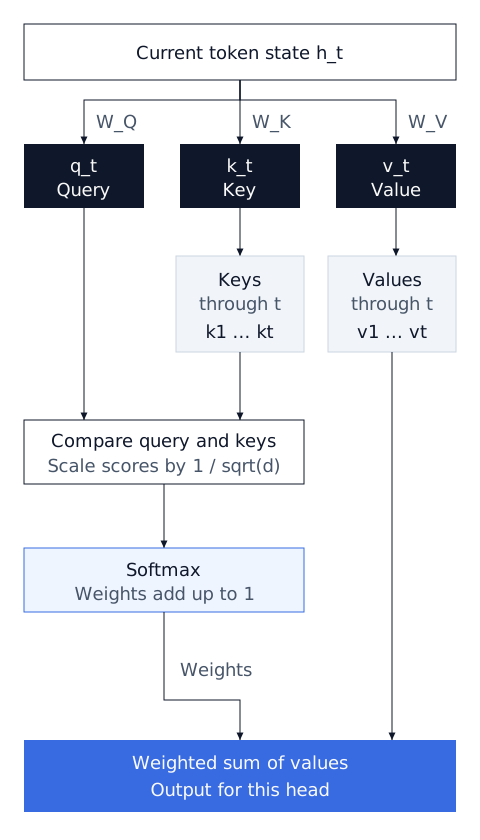
The model joins the outputs from its heads, then applies another learned transformation. More operations and layers follow. Only after the final layer does the model produce scores over its vocabulary. The engine uses those scores to choose the next token. The attention weights above describe how positions contribute to a head, rather than the probabilities of choosing output tokens.
Why keys and values stay useful
Causal attention prevents each position from reading future positions. If a sequence has five tokens and a sixth is added, the first five still depend only on the same earlier tokens and their own positions. With the same model and positional settings, their keys and values stay unchanged. Each layer can keep those vectors and reuse them.
At the sixth position, a layer computes a new query, key and value. It adds the new key and value to the stored ones. The new query is then compared with keys from all six positions, and the resulting weights combine their values. Every attention layer has its own cache because it works with a different representation of the sequence.
There is no need to keep the old queries for this step. They were used to compute the earlier positions. The new position needs its own query and the keys and values it can attend to. That is why the cache is called KV rather than QKV. The Transformers cache explanation describes this reuse at each layer.
The first pass is called prefill. It processes the prompt, builds the cache and produces the scores used to choose the first output token. Prompt positions can be processed in parallel, with a causal mask preventing each position from reading later ones. A serving engine may split a long prefill into smaller chunks.
Decode then processes the token just chosen. Its keys and values are added to the cache, and its final representation gives the scores used to choose the following token. This distinction matters. A generated token gets its own cached state when it is fed back into the model, not when it is first selected from the scores.
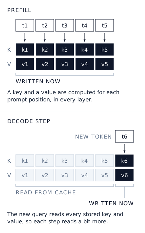
Caching saves repeated projections and the earlier layer calculations needed to produce them. It does not remove attention over the retained context. With full attention, a longer cache means more keys and values to read for each new position.
Counting memory one vector at a time
Start with one cached token in one layer and one KV head. If each vector contains numbers, its key takes numbers and its value takes another . Together they take numbers. The factor of two comes from storing both K and V.
If that layer has KV heads, it needs that pair of vectors for every head. The count becomes . With layers that all have the same shape and keep separate caches, it becomes numbers per token.
Next, multiply by the number of cached positions. This includes the prompt and the generated tokens already processed by the model. Finally, multiply by the bytes used for each number. A 16-bit cache uses 2 bytes per element. Its precision is a separate choice from the precision used for the model weights.
For several independent sequences of the same length, multiply by batch size, the number of sequences. Combining these factors gives
If sequence lengths differ, replace cached tokens times batch size with the sum of the tokens kept by all sequences. These counts assume full attention in every layer, equal key and value dimensions, and no sharing of cached data between sequences or layers.
The head count needs care. In multi-head attention, each query head has its own key and value head. In grouped-query attention, several query heads share a key and value head. Multi-query attention uses a single key and value head for all query heads. Each query head still computes its own scores, but the shared K and V only need to be stored once.
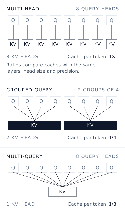
With the same layers, head dimension and precision, going from 8 KV heads to 2 cuts the cache to a quarter. A single KV head cuts it to an eighth. Read num_key_value_heads in the model configuration rather than using the number of query heads. You cannot change a trained model's attention design just by changing a serving option.
Take a hypothetical model with 32 layers, 8 KV heads, a head dimension of 128 and a 16-bit cache. One cached token across all layers costs
Multiplying this per-token cost by the number of cached positions gives
| Cached tokens | Cache size for one sequence |
|---|---|
| 1,024 | 128 MiB |
| 8,192 | 1 GiB |
| 32,768 | 4 GiB |
| 131,072 | 16 GiB |
These are calculated sizes for one sequence under the assumptions above. If eight active sequences each keep 32,768 tokens in their own cache, the cache alone needs 32 GiB, before the weights and other allocations.
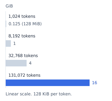
This is the logical size of the cached data. Padding, fixed-size blocks and space reserved for later tokens can make the actual allocation larger. If the model is split across GPUs, the formula counts the cache for the whole model, not its allocation on each device.
For a real example, take Qwen2.5-7B-Instruct at revision a09a354. Its configuration gives 28 layers, 4 KV heads, a hidden size of 3,584 and 28 query heads. Dividing 3,584 by 28 gives a head dimension of 128. Sliding-window attention is disabled in this configuration.
At 2 bytes per cache element, that works out to 56 KiB per token. One sequence needs 56 MiB at 1,024 tokens, 448 MiB at 8,192 tokens and 1.75 GiB at 32,768 tokens. These are calculated cache sizes, not GPU measurements. They differ from the earlier table because this model has fewer layers and KV heads.
The calculation fits in a short Rust program. It uses the configuration values above and needs no extra crates, model weights or GPU.
fn main() {
    let layers = 28_u64;
    let kv_heads = 4;
    let head_dimension = 3_584 / 28;
    let bytes_per_element = 2;
    let bytes_per_token = 2 * layers * kv_heads * head_dimension * bytes_per_element;
    let lengths = [1_024, 8_192, 32_768];
    let mut total_bytes = 0;

    for tokens in lengths {
        let bytes = bytes_per_token * tokens;
        total_bytes += bytes;
        println!("{tokens} tokens -> {} MiB", bytes / (1024 * 1024));
    }

    println!("Total -> {} MiB", total_bytes / (1024 * 1024));
}
Save the code as estimate.rs. With Rust installed, compile and run it from the same folder.
rustc estimate.rs -o estimate && ./estimate
Each length represents one sequence running at the same time. The program prints 56, 448 and 1,792 MiB, then their combined total of 2,296 MiB. All three lengths fit within the 32,768 positions in the linked configuration. Longer contexts require a separate setup and are outside this example.
Ways to shrink or share the cache
Cache quantization stores keys and values with fewer bits, for example 8 instead of 16, which halves the memory per element. It can cost some output quality, and some kernels need extra work to read the compressed format. Test both accuracy and speed on your own workload before turning it on.
Paging, as in vLLM's PagedAttention, splits the cache into fixed-size blocks instead of one long reserved region per sequence. It reduces unused gaps and space set aside for tokens that have not arrived. It changes how memory is managed. The vectors needed by full attention still have to be stored.
Sliding-window attention limits how far back certain layers look. For those layers, the engine can discard positions outside the window. The number of retained tokens stops growing once the window is full. A model with both sliding and full-attention layers needs a separate count for each type.
Prefix caching lets requests reuse cached data for an identical beginning, such as a long system prompt, under the same model settings. An engine that shares those cache blocks can avoid storing a separate copy for every request. Private request data must still be kept isolated. The Transformers cache documentation also covers fixed-size, growing and quantized caches.
What to measure under load
The cache shares memory with the model weights, temporary activations and working space used by GPU kernels. Activations are the intermediate results produced during a forward pass. The allocator may also hold unused memory for later work. A calculation based only on the model file leaves out these allocations as well as the cache.
Continuous batching adds new requests to a running batch as others finish. Count the token state held by all active sequences, including requests waiting between steps. The number of tokens processed in one step and the total number retained in caches are different quantities.
An open chat does not always keep a cache on the GPU. After a request ends, the server may release its cache. A later request may need to process the conversation again, unless the server can reuse a saved prefix. Count the state the engine actually keeps, rather than every conversation stored by the application.
A server sized around the average conversation can run out of cache space when a few long requests overlap. Record memory after the model loads, after a long prefill and during generation. Then repeat with several requests running together, using the range of lengths your application handles. Leave some memory free for other work.
Compare what the framework reports with what the process and the device report. In PyTorch, torch.cuda.memory_allocated() counts memory used by live tensors. torch.cuda.memory_reserved() also includes memory the allocator keeps for later. nvidia-smi shows GPU memory used by the process, which can include allocations outside PyTorch's allocator. These views count different things, so none is a direct measure of the cache alone.
Some engines reserve their GPU cache pool at startup. The reported memory can then stay almost flat as requests fill that pool. Watch the share of cache blocks in use as well. When space runs out, vLLM can pause requests and later recompute their state. That can increase response time without a new GPU allocation or an out-of-memory error.
Run a test with several long requests at once. Record cache use, any paused or recomputed requests, and response times alongside GPU memory. Use that result to set your serving limits, then repeat the test when the model, cache precision or expected request lengths change.